


Description
This application note explains the minimum hardware and software requirements for obtaining an angular position measurement from a Fredericks electrolytic tilt sensor.
Basic Design and Sensor Excitation
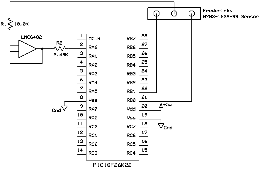
Figure 1 shows the major components required to create a functioning tilt measurement unit using an electrolytic tilt sensor.

As you will see later on, it is important to avoid direct current to the sensor. We therefore suggest the use of an operational amplifier with high input impedance such as the LMC6482 from Texas Instruments. This will limit current leakage to ground and in turn, direct current to the sensor. Figure 2 shows the circuit equivalent of a single axis electrolytic tilt sensor.

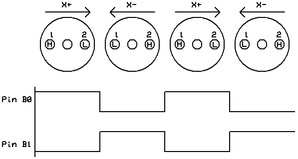
Let’s continue with the excitation signal for the sensor. The excitation signal is provided by the microprocessor with the simplest case being a single axis sensor. A single axis sensor requires two output ports of the microprocessor which are connected to the outer pins of the sensor. The ports are toggled with a 50% duty cycle and a period of between 200 and 1000 hertz. See Figure 3.
Precise timing in software is required to maintain a 50% duty cycle to prevent asymmetry in the sensor excitation signal. See Figure 4. Asymmetry is defined as direct current to the sensor which causes drift and ultimately permanent and irreversible damage to the sensor. This can be explained chemically; direct current causes electrolysis to take place, eventually rendering the sensor inert.
Let’s examine the process of creating an excitation signal in software for a PIC18F microprocessor using the CCS PCW C Compiler. These instructions will differ significantly depending on your specific microprocessor and compiler. We’ll start by defining which pins will be used for output. We will use PORTB for output so we will need to define it as such. This is accomplished by setting the 8 bit data direction register, called TRISB. Bits in TRISB set to 0 will define the corresponding PORTB pin as an output, so we will use the following line of code to use all PORTB pins for output:
set_tris_b(0b00000000); |
In order to quickly change the PORTB pin values, we will need to access it in memory. On this particular microprocessor, PORTB is a special function register (SFR) which is located at memory address 0xf81. We will therefore store the location of PORTB in a variable to allow easy access. This is accomplished with the following line of code:
#byte port_b = 0xf81; |
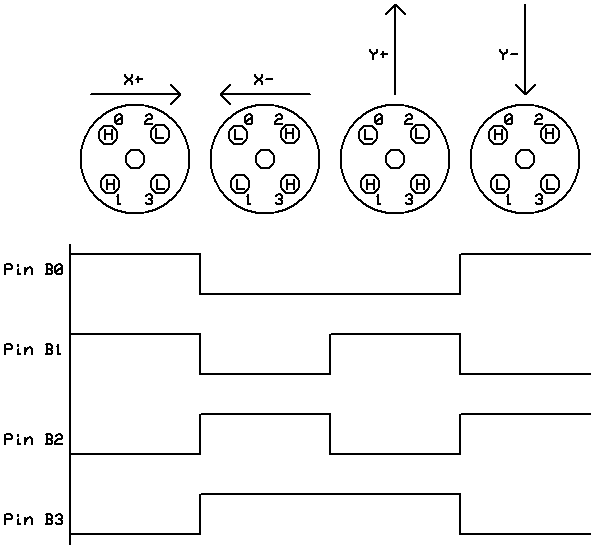
Each bit in port_b now corresponds to a pin on the chip. The most significant bit is pin B8 and the least significant bit is pin B0. Let’s assume a single axis sensor is connected to pins B0 and B1. See Figure 3. If you are using a dual axis sensor, let’s assume it is connected to pins B0, B1, B2, and B3.
For a single axis sensor, there are two states for the excitation signal. See Figure 4. To mimic this timing diagram, the two states can be stored in an array of 8 bit numbers. This is accomplished with the following line of code:
int8 output_arr[2] = { 0b00000010, 0b00000001 };
|
For a dual axis sensor, there are four states for the excitation signal. See figure 5. To mimic this timing diagram, the four states can be stored in an array of 8 bit numbers. This is accomplished with the following line of code:
int8 output_arr[4] = { 0b00000011, 0b00001100, 0b00001010, 0b00000101 };
|
Timers are a commonly used tool to generate interrupts at precise intervals in software and they can be used to easily generate an excitation signal. It is important that we use a high priority interrupt so that the excitation signal maintains a 50% duty cycle. The following code creates a high priority interrupt which toggles the ports to generate an excitation signal for a dual axis sensor:
int isr_counter = 0;

#int_timer1 HIGH
void timer1_isr(void) {
     set_timer1(64535);
     port_b =  output_arr[ (isr_counter++) % 4];    // this is for a dual axis sensor
}
|
In this example, timer1 is a 16 bit counter (0 to 65535). This means that it will count up from the value set by set_timer() and when it overflows (reaches 65535), an interrupt will be generated and the code within the timer1_isr() function will be executed. The amount of time that it takes to overflow is defined by a variety of factors including the microprocessor clock speed and the timer1 setup parameters, among others. It is important to maintain an interrupt time of between 1 and 5 milliseconds to ensure proper excitation of the sensor. Refer to the manual of your individual microprocessor for this information.
The port toggling works by using the modulus function. Each time an interrupt is generated, isr_counter is incremented and modulus 4 is performed on it. This essentially makes a counter that counts from 0 to 3, incrementing with each interrupt. This accesses each of the four states stored in output_arr that comprise the excitation signal.
Sensor Output
Now that we’ve created an excitation signal, let’s examine the sensor’s output. The output is an analog voltage referenced to the excitation voltage. The output must be read in phase with the excitation signal. It is suggested to take multiple samples during each of the four states (two states for a single axis sensor).
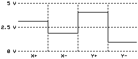
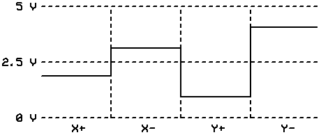
The waveform in Figure 6 shows an example output from the analog to digital converter connected to the output of a dual axis sensor. This particular output indicates a positive tilt angle for both the x and y axis. See Figure 7 for an output indicating a negative tilt angle.
In order to read the output we will need to use the microprocessor’s analog to digital converter (ADC). Looking at Figure 3 we will need to set up pin A0 as an ADC input and then set the current ADC port to pin A0. We can then execute the following code to read the output from a dual axis sensor in phase with the excitation signal:
int samples = 0;
int index = 0;
int xpos[8], xneg[8], ypos[8], yneg[8] = {0,0,0,0,0,0,0,0};

while(true) {
     while( (isr_counter % 4) != 0 );
     while( (isr_counter % 4) == 0 ) {          // loop to read x positive state
          delay_us(100);
          if(index <= 7)
               xpos[index] = Read_ADC();
          index++;
     }
     index = 0;

     while( (isr_counter % 4) != 1 );
     while( (isr_counter % 4) == 1 ) {          // loop to read x negative state
          delay_us(100);
          if(index <= 7)
               xneg[index] = Read_ADC();
          index++;
     }
     index = 0;

     while( (isr_counter % 4) != 2 );
     while( (isr_counter % 4) == 2 ) {          // loop to read y positive state
          delay_us(100);
          if(index <= 7)
               ypos[index] = Read_ADC();
          index++;
     }
     index = 0;

     while( (isr_counter % 4) != 3 );
     while( (isr_counter % 4) == 3 ) {          // loop to read y negative state
          delay_us(100);
          if(index <= 7)
               yneg[index] = Read_ADC();
          index++;
     }
     index = 0;

     // data processing and analysis would then be done here
}
|
As you can see, within each state of the excitation signal we are collecting 8 samples with a 0.1 ms delay between samples. These samples can then be averaged in the data analysis code to provide a more stable and accurate result. By referencing the isr_counter we are able to ensure that the readings are taken in phase with the excitation signal.
Deriving Tilt Angle
The tilt angle of the sensor can be derived by comparing the difference between the voltages for each excitation state:
X axis tilt = (X+) – (X-)
Y axis tilt = (Y+) – (Y-)
Let’s say we have a 16-bit (0 to 65535 counts) analog to digital converter reading the output from a ±20° dual axis sensor. This means that our range of output is ±65535 counts using the definitions of X and Y axis tilt above. Let’s examine the following output for one cycle:
X+ = 45535
X- = 20000
Y+ = 30000
Y- = 35535
We can then conclude the following:
X axis tilt = +25535
Y axis tilt = -5535
Now to convert this into an angle measurement:
±65535 counts = 131070 counts range
±20° = 40° range
131070 counts / 40° = ~3277 counts/°
25535 counts / (3277 counts/°) = ~+7.79° x axis tilt
-5535 counts / (3277 counts/°) = ~-1.69° y axis tilt
Mechanical Considerations when Deriving Tilt Angle
All sensors have mechanical tolerances and their operating specifications often only indicate a portion of their total range. Additionally, the above calculation assumes a linear, symmetrical, and centered output from the sensor and this is typically not the case. It is therefore important to characterize the specific type of sensor you are using in your application in order to derive the true tilt position.
For example, let us consider a single axis ±25° electrolytic sensor. Figure 8 shows the mechanical functionality of this tilt sensor:

Let’s say this time that we have a 12-bit (0 to 4095 counts) analog to digital converter reading the output from the sensor. This means that our range of output is ±4095 counts using the definition of X axis tilt in the previous section. In order to individually characterize the sensor, we would first tilt it to -25° and take a reading. Let’s examine the following output for one cycle at -25° tilt:
X+ = 400
X- = 3700
X axis tilt at -25° = 400 – 3700 = -3300
We would then tilt the sensor to +25° and again take a reading. Let’s examine the following output for one cycle at +25° tilt:
X+ = 3700
X- = 400
X axis tilt at +25° = 3700-400 = 3300
We can then do the following calculations:
3300 – (-3300) = 6600 counts range
±25° = 50° range
6600 counts / 50° = 132 counts/°
Knowing the number of counts per degree allows you to easily convert a reading from the analog to digital converter to an angular position. Further compensation for linearity, symmetry, and zero position will significantly increase the accuracy of angular calculations.
Software Considerations
As with all software, there are many different ways to accomplish the same goal. This document simply presents one example of how electrolytic tilt sensor signal conditioning can be achieved through the use of a specific microprocessor and compiler.